Towards scalable, inductive, intrinsic diffusion geometry
Iolo Jones
University of Oxford & AITHYRA
How is geometry dynamic?
Experiments observe systems under change. There is
•… an underlying process (dynamics)
•… that is constrained (geometry)
Classical geometry: rigid and flat
This geometry is the study of static structure
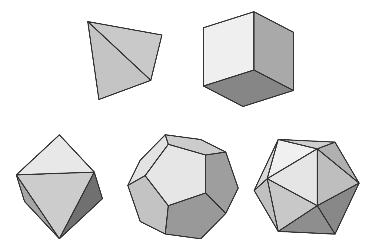
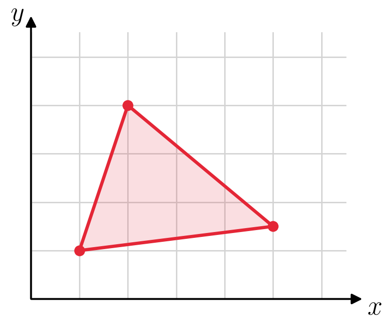
Platonic solids
Euclidean geometry
Calculus
Language for describing change and dynamics
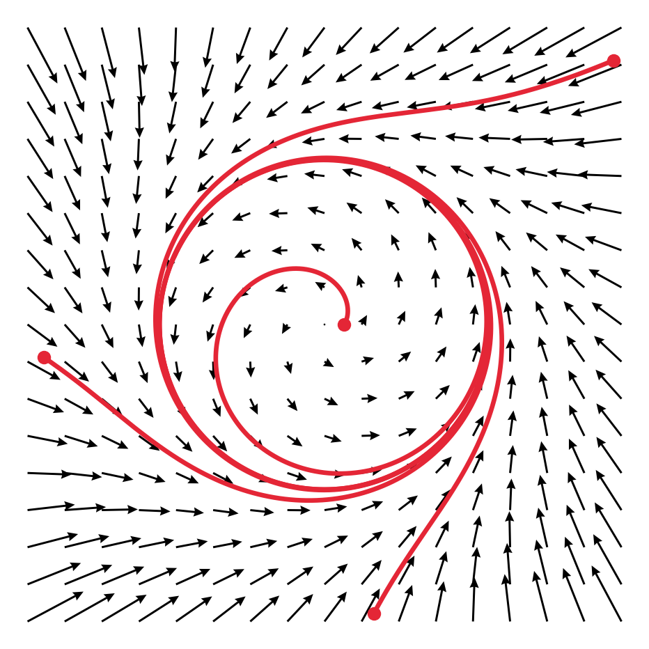
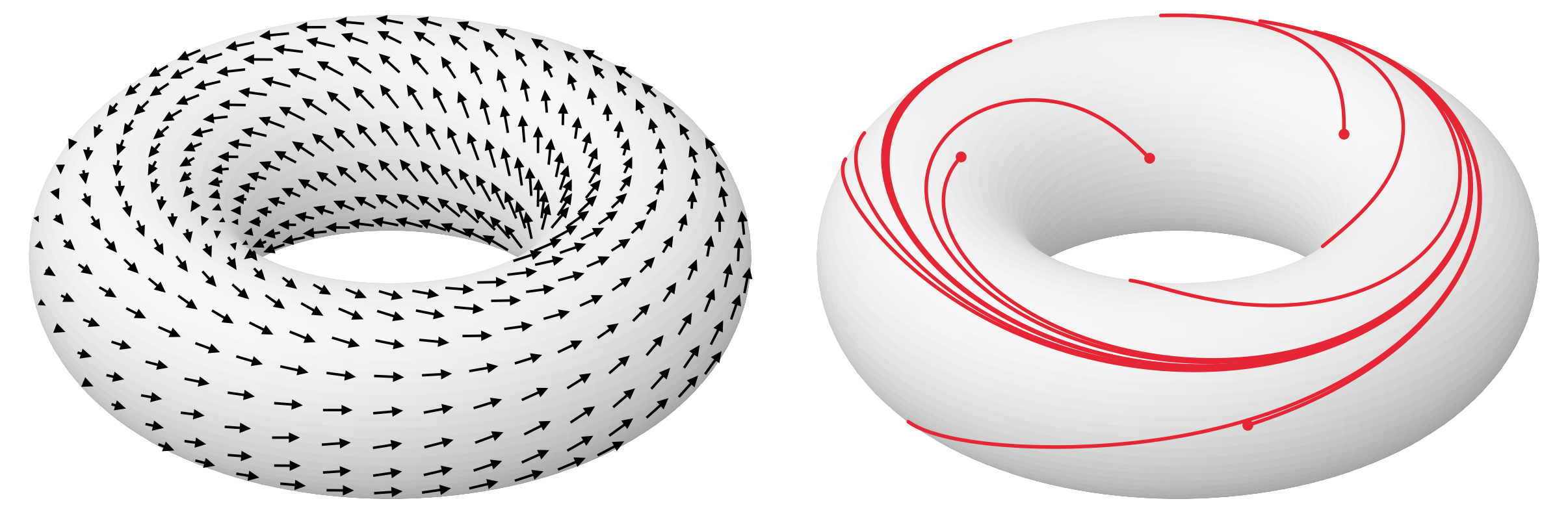
Riemannian geometry
Uses calculus to study more general geometries (manifolds)
This geometry is the study of change across structure
Problem 1: how can we estimate it from data?
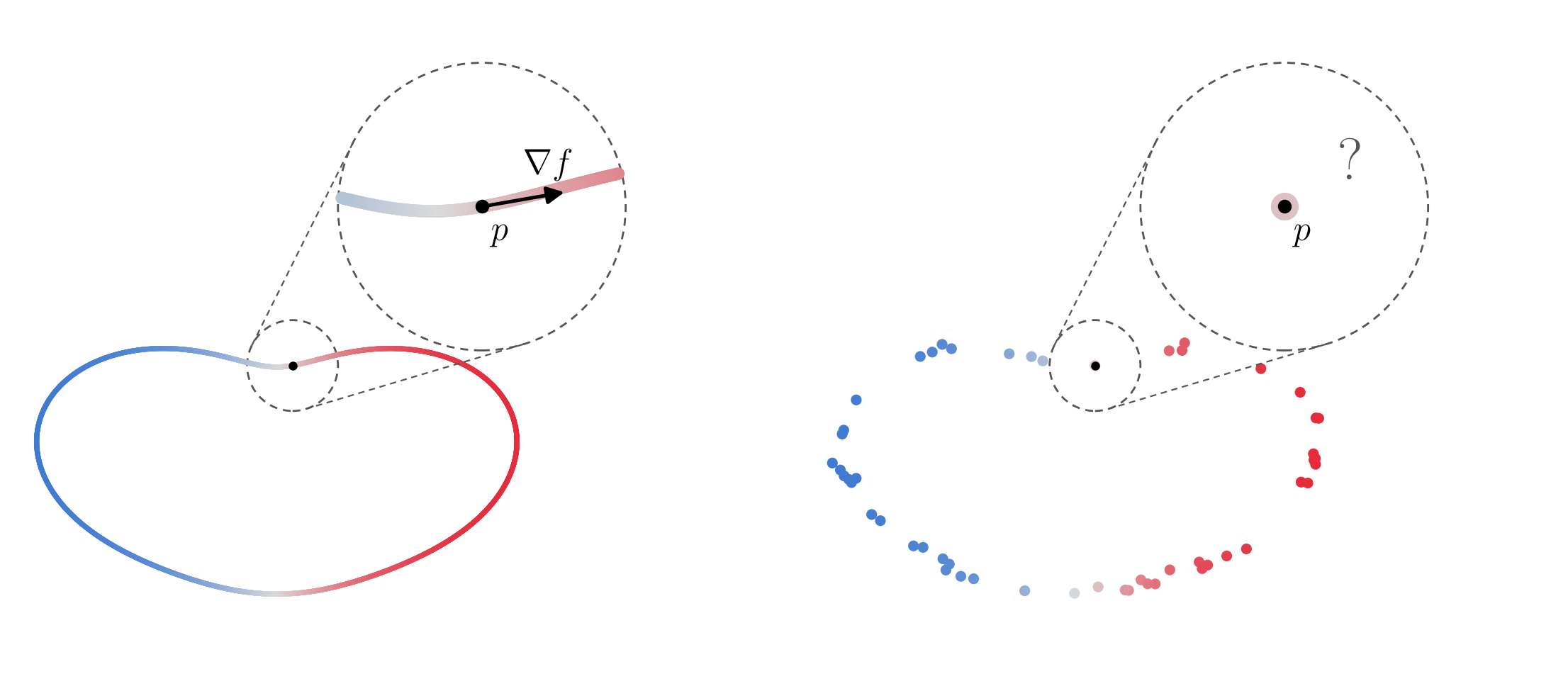
\(\displaystyle \frac{df}{dx}(p) = \lim_{h\to 0}\frac{f(p+h)-f(p)}{h}\)
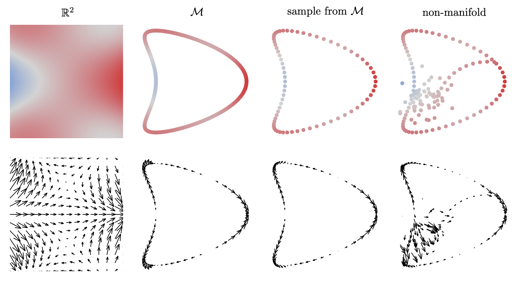
Data has gaps.
perfectly homogeneous:
manifold
intersection points:
non-manifold
variable dimension:
non-manifold
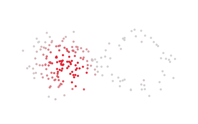
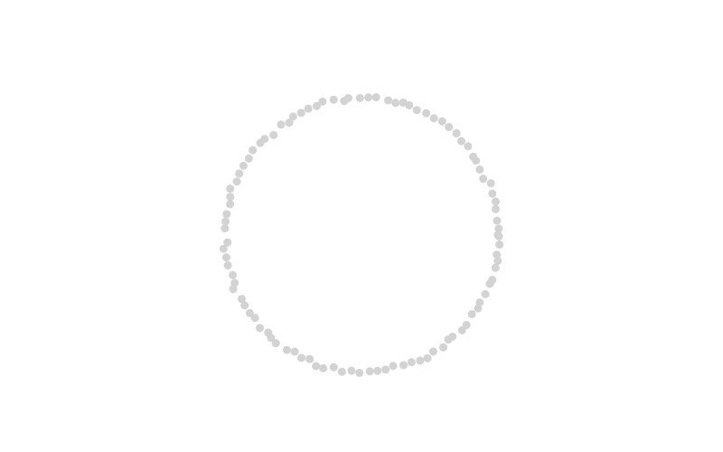
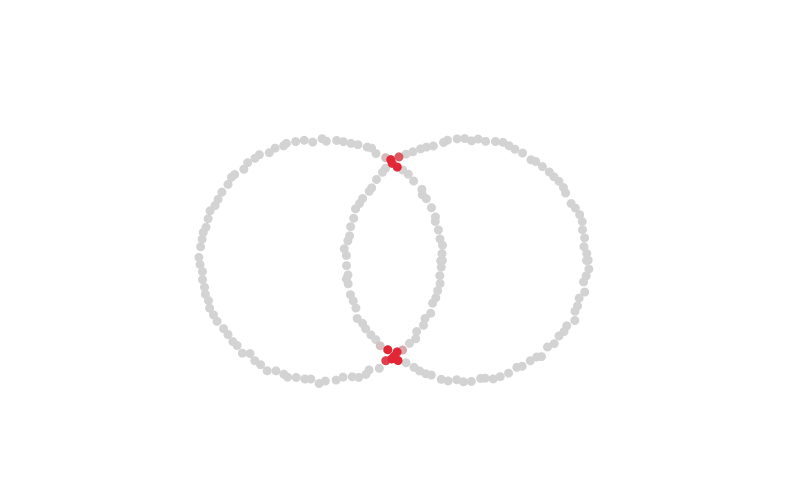
Problem 2: Riemannian geometry is not a general enough language
The manifold assumption is too rigid – real data are heterogeneous
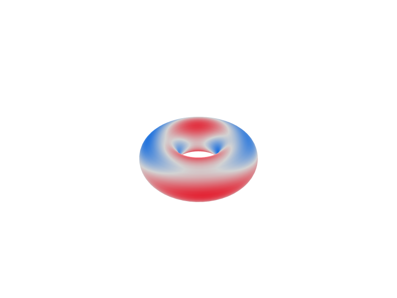
Calculus on different spaces. How can we apply it to geometric/spatial data?
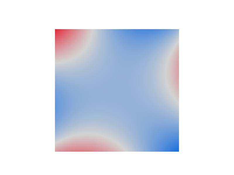
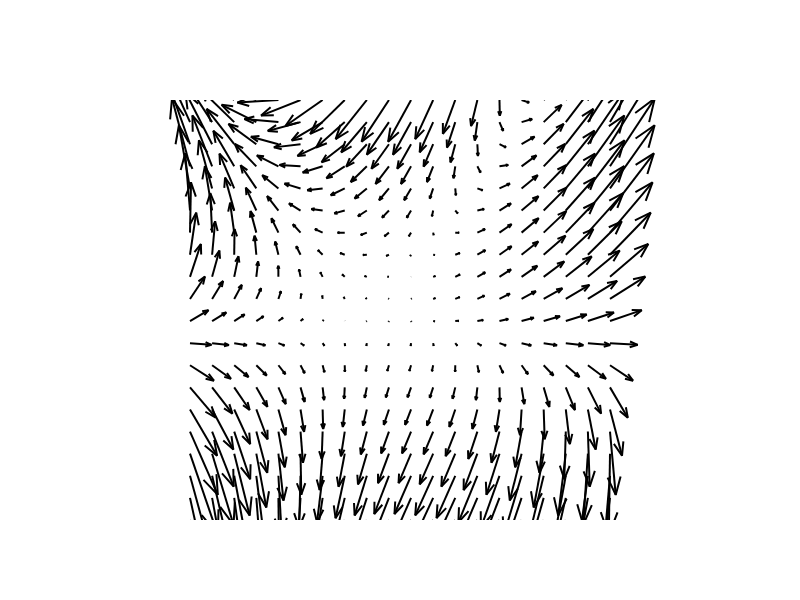
Euclidean space:
vector calculus
Manifolds:
Riemannian geometry
Point clouds:
??
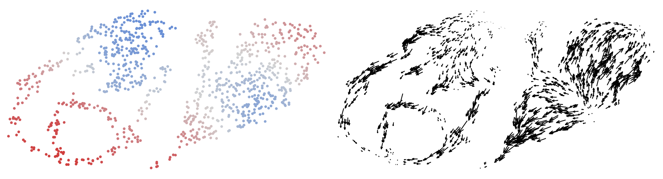
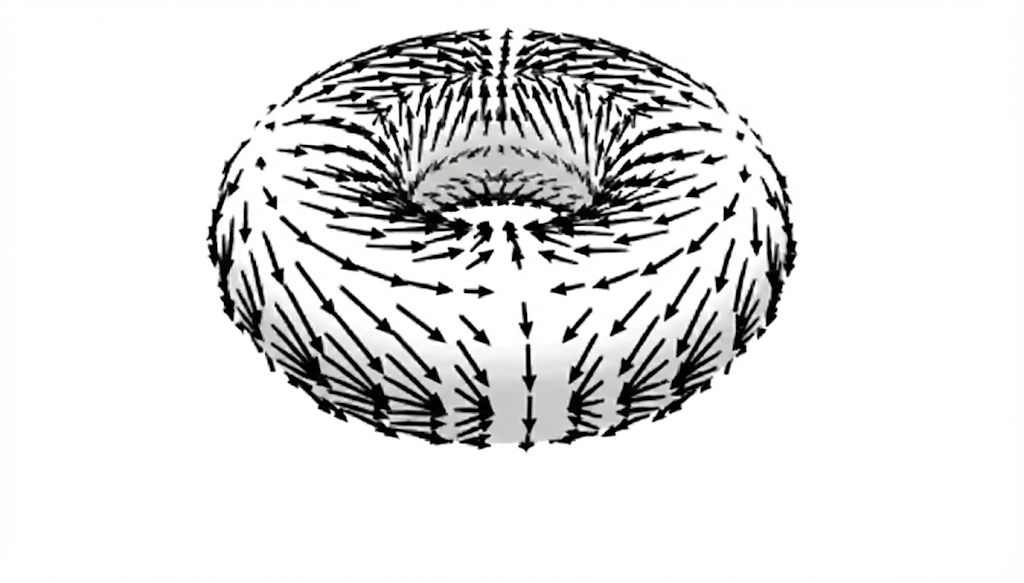

Diffusion geometry: the geometry is the dynamics
•On manifolds, the geometry/calculus is captured by the Riemannian metric: the dot product of vector fields \(g(X,Y) = X\cdot Y\)
•We can interpret this as the local covariance of a diffusion process
\(\displaystyle g(\nabla f,\nabla h)(p) = \lim_{t\to 0}\frac{1}{2t}\,\mathrm{Cov}\big[f(X_t),\,h(X_t)\;:\;X_0 = p\big]\)
where \(X_t\) is Brownian motion
•This is called the carré du champ (CDC) – it exists on more general spaces than manifolds
\(\displaystyle \Gamma(f,h)(p) = \lim_{t\to 0}\frac{1}{2t}\,\mathrm{Cov}\big[f(X_t),\,h(X_t)\;:\;X_0 = p\big]\)
where \(X_t\) is a general diffusion process
(Jones 2024)
Computing the carré du champ from diffusion on the data
We use a data-driven analogue of this diffusion relationship:
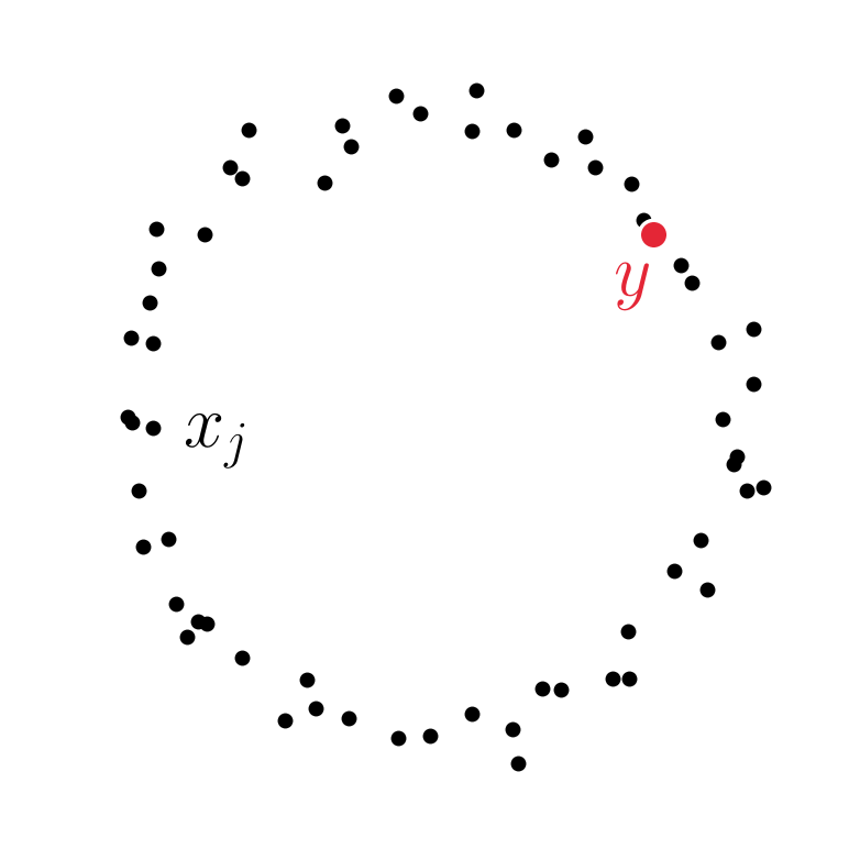
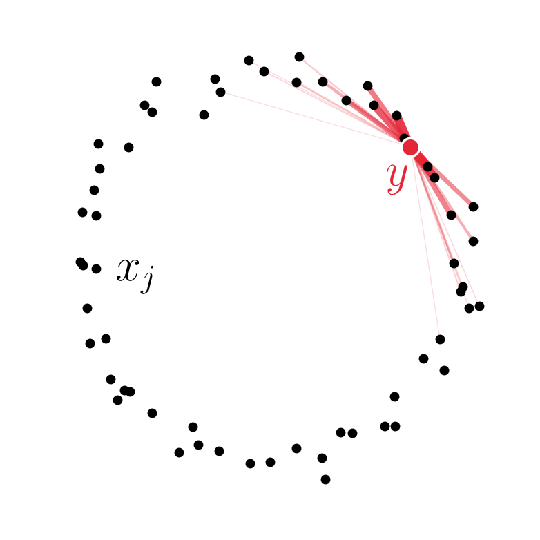
1.Compute the heat kernel from a point y to each data point xj:
2.Normalise to get a Markov chain (a discrete diffusion process):
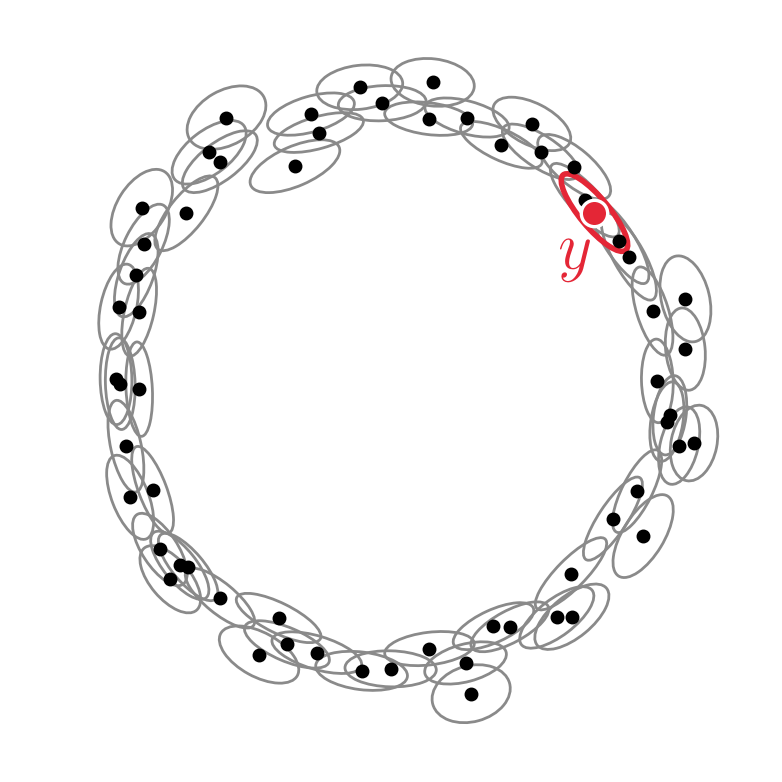
3.The carré du champ at y is the local covariance of one step:
(Jones 2024; Jones & Lanners 2026)
\(\displaystyle p_t(y,x_j) = \exp\left(-\frac{\|y-x_j\|^2}{4t}\right)\)
\(\displaystyle \hat{p}_t(y,x_j) = \frac{p_t(y,x_j)}{\sum_{k=1}^n p_t(y,x_k)}\)
\(\displaystyle \Gamma(f,h)(y) = \frac{1}{2t}\sum_{j=1}^n \hat{p}_t(y,x_j)\,\big(f(x_j)-f(y)\big)\big(h(x_j)-h(y)\big)\)
Example: visualising the gradient of a function
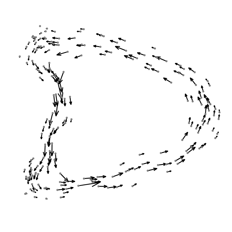
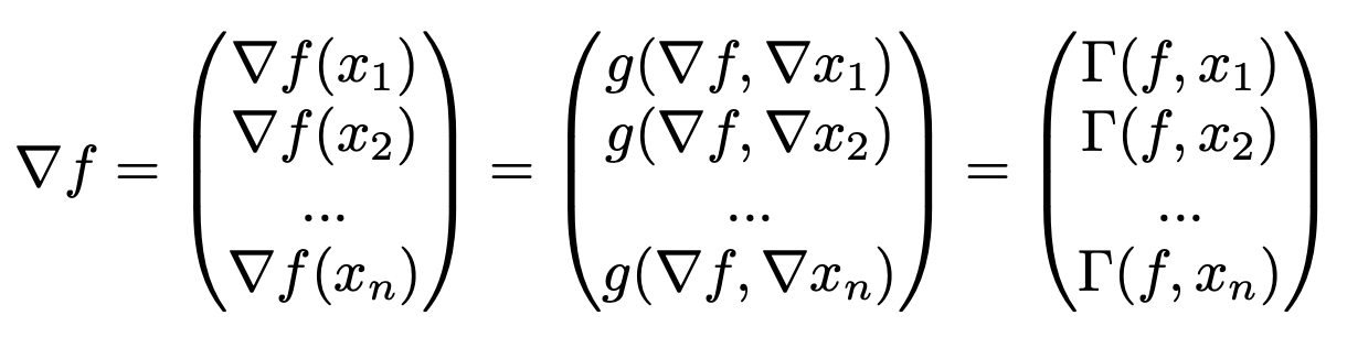
The gradient of a function is a vector field. We can visualise it as a collection of arrows
We estimate these CDC terms using our kernel covariance method.
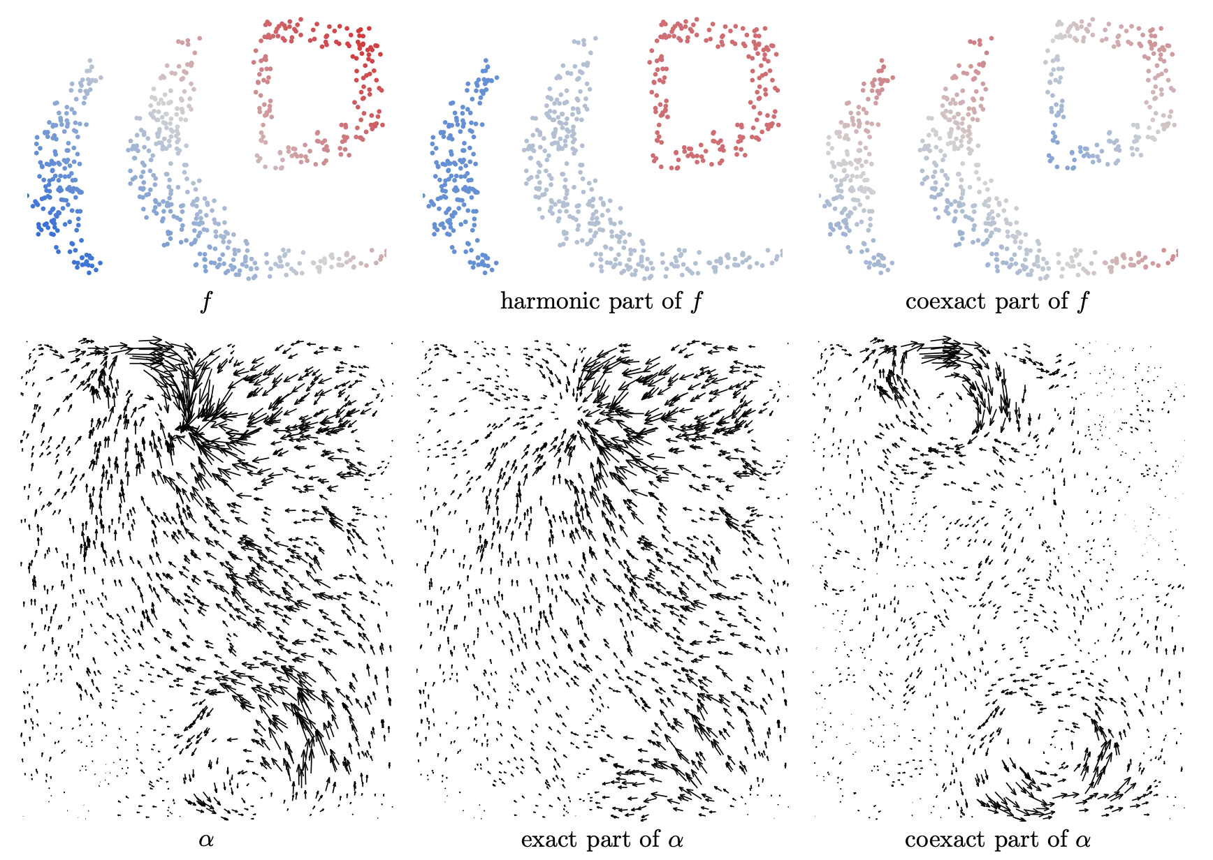
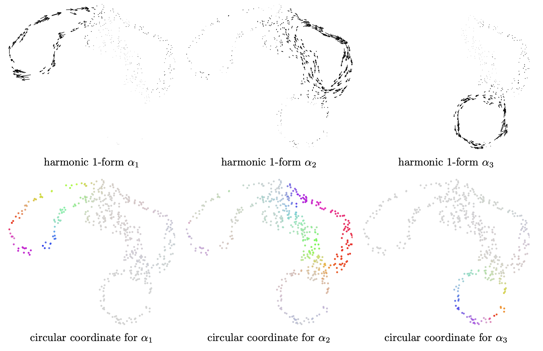


\(\text{harmonic 1-form } \alpha_1\)
\(\text{harmonic 1-form } \alpha_2\)
\(\text{harmonic 2-form } \beta\)
\(\text{harmonic 1-form } \alpha_1\)
\(\text{harmonic 1-form } \alpha_2\)
\(\text{harmonic 2-form } \beta\)
Solving spatial PDEs: heat and wave equations
Vector field flows

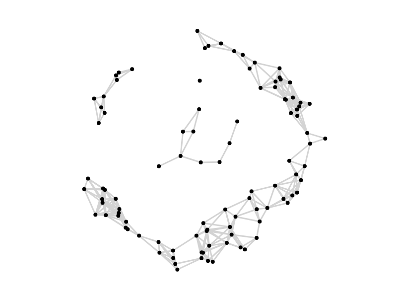
Graph / kernel methods have limits.
•Graph / kernel methods dominated ML until ~2012
•Deep learning then took off. Why?
Issue 1: curse of dimension
Kernels involve distances between pairs of points.
These are not informative in high dims.
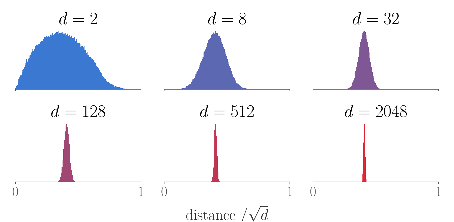
![Histograms of pairwise distances (divided by sqrt d) between uniform random points in [0,1]^d for d = 2, 8, 32, 128, 512, 2048: they concentrate as d grows](/assets/talks/scalable-inductive-intrinsic/s21-5b56c94fe6.png)
Issue 2: scalability
Recall the kernel estimate of the carré du champ:
These sums over the whole dataset are too expensive! The cost grows like n2 in high dimensions.
\(\require{color}\definecolor{dgred}{RGB}{228,38,54}\displaystyle \Gamma(f,h)(y) = \frac{1}{2t}\textcolor{dgred}{\sum_{j=1}^n} \frac{p_t(y,x_j)}{\textcolor{dgred}{\sum_{k=1}^n}\, p_t(y,x_k)}\,\big(f(x_j)-f(y)\big)\big(h(x_j)-h(y)\big)\)
Issue 3: poor generalisation beyond the training data
•Graph methods are transductive: they explicitly reference the training data based on proximity
•Neural networks are inductive: they learn general purpose features that apply elsewhere
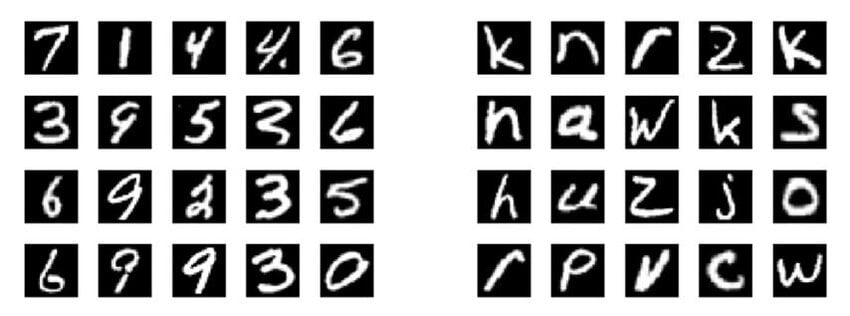
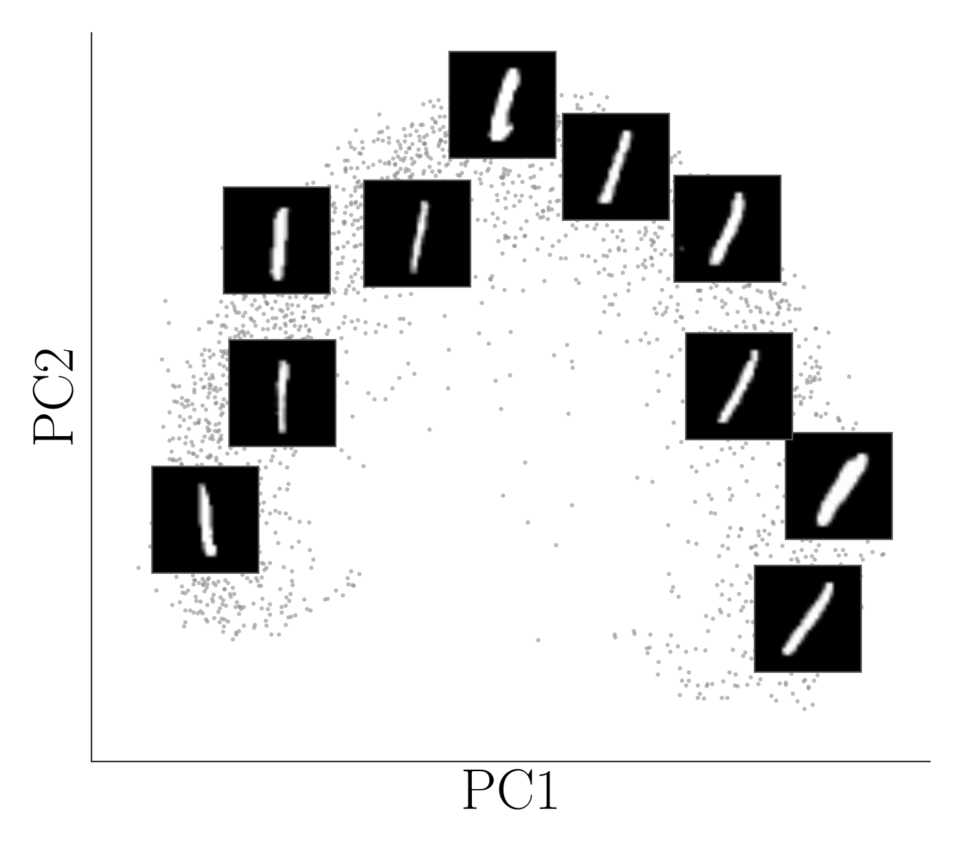
MNIST digits
EMNIST letters
Replacing the kernel with a training loss
•The kernel carré du champ matrix is an average over nearby data:
•Train a neural network Γθ with a loss:
•Theorem: \(\mathcal{L}_{\mathrm{cond}}(\theta) = \mathcal{L}_{\mathrm{true}}(\theta) + \text{constant}\)
So the two losses have the same minimiser and gradients
•One pair of points per step: no sums over the data.
•The kernel is implicit in the sampling not explicit in the kernel.
(Bamberger, Gosztolai, Vandergheynst, Bronstein, Jones 2026)
\(\displaystyle \Gamma(y) = \frac{1}{2t}\sum_{j=1}^n \hat{p}_t(y,x_j)\,(x_j-y)(x_j-y)^\top\)
\(\displaystyle \phantom{\Gamma(y)} = \mathbb{E}\left[\frac{(Y-X)(Y-X)^\top}{2t}\;\middle|\;Y=y\right],\qquad X\sim\text{data},\quad Y\sim\mathcal{N}(X,2t\boldsymbol{I})\)
\(\displaystyle \hspace{3.6cm}\llap{\text{true loss:}}\quad\mathcal{L}_{\mathrm{true}}(\theta) = \mathbb{E}_{Y}\,\big\|\Gamma_\theta(Y) - \Gamma(Y)\big\|^2\)
\(\displaystyle \hspace{3.6cm}\llap{\text{conditional loss:}}\quad\mathcal{L}_{\mathrm{cond}}(\theta) = \mathbb{E}_{X,Y}\left\|\Gamma_\theta(Y) - \frac{(Y-X)(Y-X)^\top}{2t}\right\|^2\)
MNIST image geometry

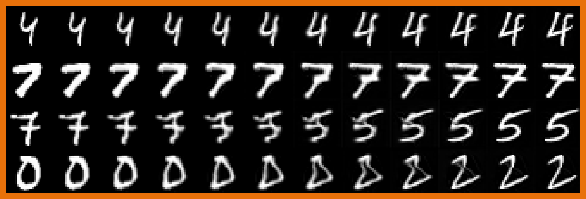
Interpolating paths (in and out of distribution)
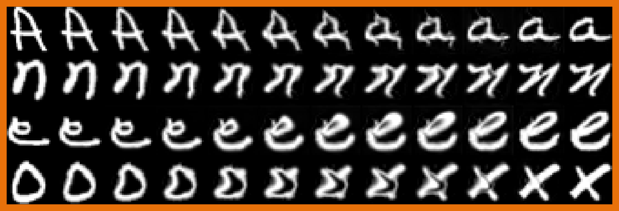

(Lecha, Bronstein,
Jones 2026)
MNIST ‘tangent vectors’


What about intrinsic geometry?
•Most experimental data is an arbitrary observation of an unknown underlying process. The observation can distort the geometry.
•E.g. two satellite images being ‘close’ as images does not mean the two weather systems are related
•How can we disentangle the true geometry of the process?
(Lecha, Bronstein, Jones 2026)
Intrinsic Geometry Matching
Kernels imply a notion of affinity/proximity between points.
Idea: forget that and use consecutive time points as ‘perturbations’, i.e. sample from the (unknown) true kernel of the system.
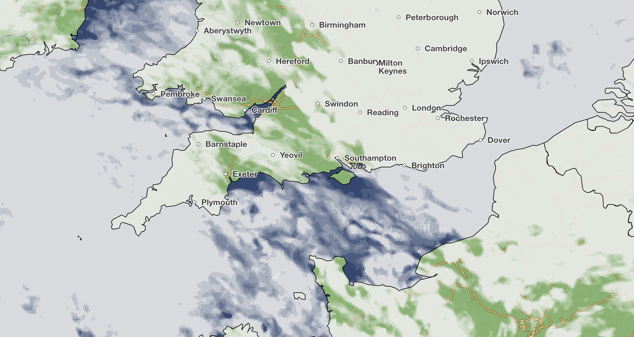
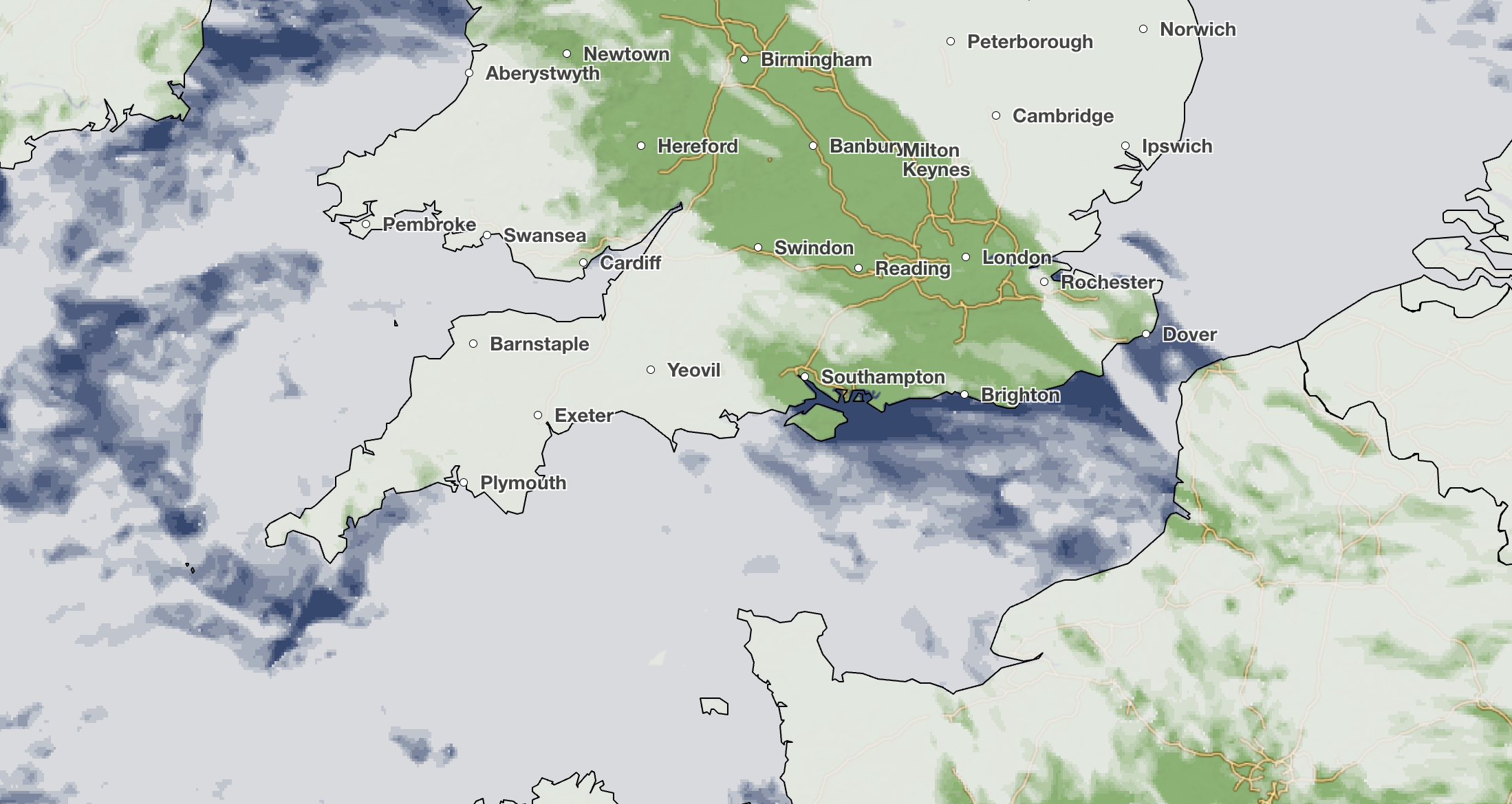
\(\displaystyle X_t\)
\(\displaystyle X_{t+1}\quad\text{(1 hour later)}\)
(Lecha, Bronstein, Jones 2026)
Intrinsic Geometry Matching
•Replace the Gaussian noise with the system's own perturbations:
•The kernel is now the true kernel of the system: it can be unknown, and is only implicit in the data
\(\require{color}\definecolor{dgred}{RGB}{228,38,54}\displaystyle \begin{aligned}\text{RMM:}\quad &\mathbb{E}\left\|\Gamma_\theta(Y) - \frac{(Y-X)(Y-X)^\top}{2t}\right\|^2, &&Y \sim \mathcal{N}(X,2t\boldsymbol{I})\\[6pt] \text{IGM:}\quad &\mathbb{E}\left\|\Gamma_\theta(X) - \frac{(Y-X)(Y-X)^\top}{2t}\right\|^2, &&\textcolor{dgred}{Y = \text{the system observed a time } t \text{ after } X}\end{aligned}\)
E.g. videos imply the ‘natural’ image geometry
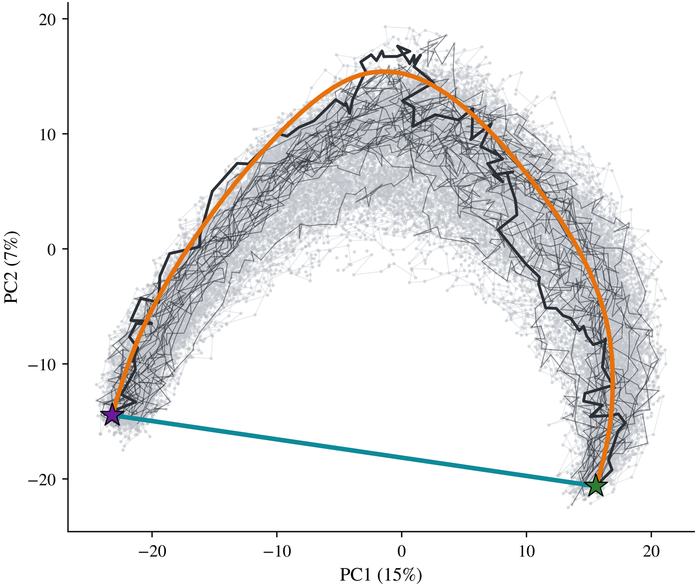
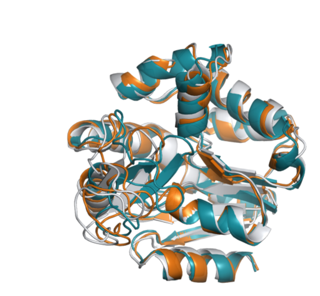
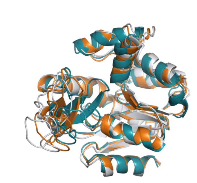
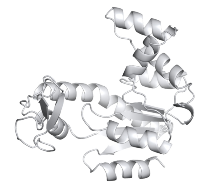
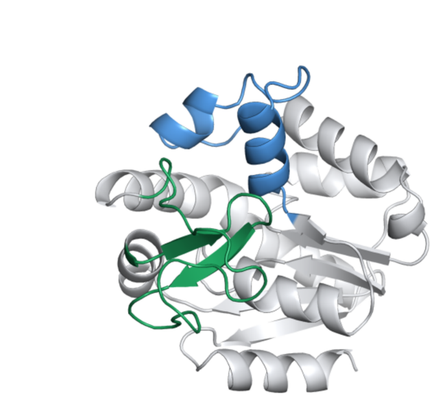
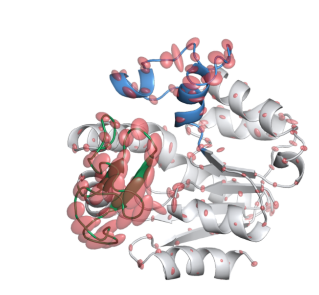
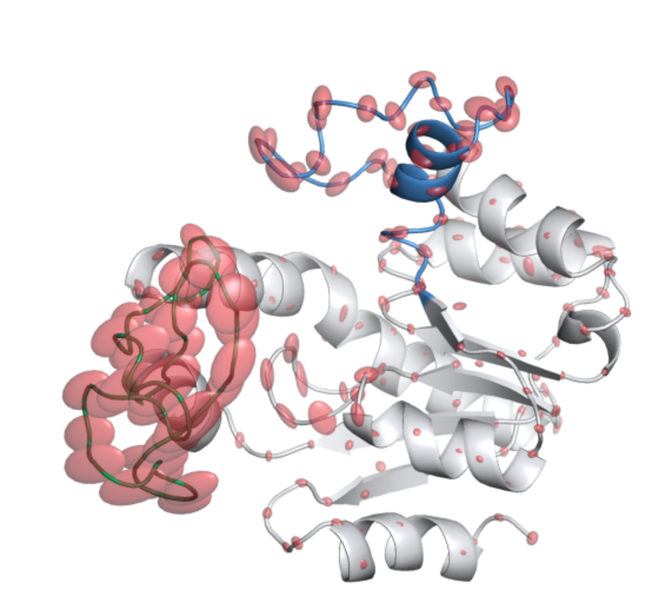
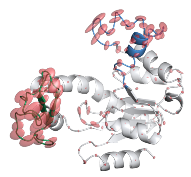
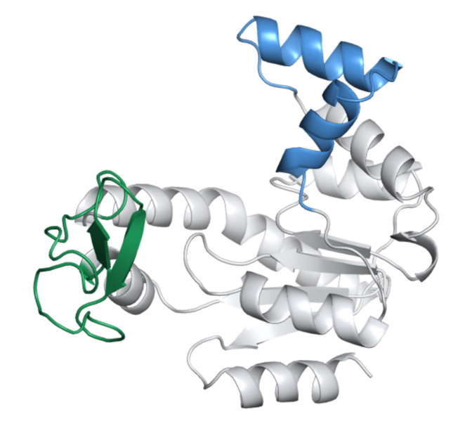
Recovering protein transition path
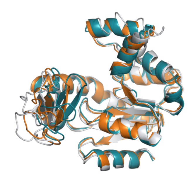


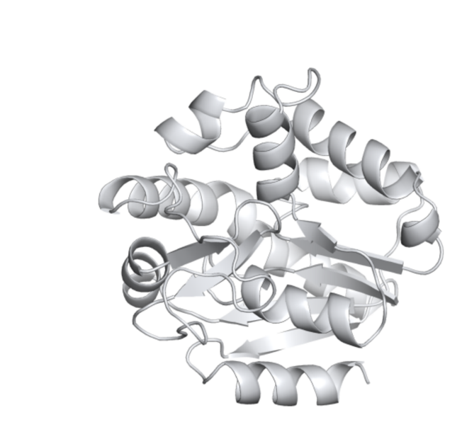
Conformational dynamics: visualising the CDC in molecular coordinates
Summary
•Experiments often observe constrained dynamics: geometry a natural language. But what’s the right geometry?
•Diffusion geometry: Riemannian tools without the manifold assumption, computable from data.
•Neural networks make it scalable and inductive.
•Learning from the system's own transitions recovers its intrinsic geometry.
References.
Theory:
•Diffusion Geometry
Iolo Jones, 2024
Graph methods:
•Manifold Diffusion Geometry: Curvature, Tangent Spaces, and Dimension
Iolo Jones, 2024
•Computing Diffusion Geometry
Iolo Jones & David Lanners, 2026
Deep learning:
•Riemannian Metric Matching for Scalable Geometric Modeling of Distributions
Jacob Bamberger, Adam Gosztolai, Pierre Vandergheynst, Michael Bronstein, Iolo Jones, 2026
•Intrinsic Geometry Matching: learning observation-equivariant process geometry
Manuel Lecha, Michael Bronstein, Iolo Jones, 2026